Connected to our work on continuous ecological monitoring, we set up bioacoustics recorders at four sites in Delhi to continuously collect audio data. This blog outlines some analysis pipelines we have built to understand the data and we look forward to feedback to improve this further.
Site description
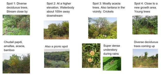
The sites themselves were visibly quite diverse and we hoped we would see differences in the fauna at these sites.
Bird species identification
We therefore first ran the audio through BirdNet to get bird species identifications, and also compared them with eBird lists from the location to see if the ML models were making spurious detections. Indeed, we found several species not on eBird but identified by BirdNet, with a low detection frequency, quite likely to be misclassifications, and removed them from our analysis. Sticking to high frequency occurrences, and only those species reported on eBird lists for the area, we then proceeded with further analysis and computed the number of detections of a species per hour, per spot, using data from about two weeks of recording. The chart below helps give a sense of the prevalence of different bird species at a spot.
Bird behaviour analysis
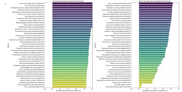
We also did an interesting analysis of bird behaviour, which we termed as temporal and spatial stickiness. Temporal stickiness is an indicator for how regular a bird species is in its vocalizations at different times of the day. We do this by computing a ranking of vocalizations of a bird species in each hour, and find the rank correlation across consecutive pairs of days. We then rank the bird species in terms of which ones are the most regular day-on-day on the intensity of their activities.
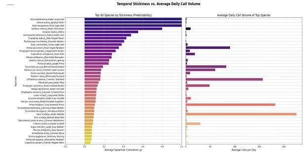
Similarly, we built an indicator for spatial stickiness to rank bird species in terms their preference for different sites, i.e. do they consistently day-on-day prefer one site over the other or do they roam around.
Site characterization
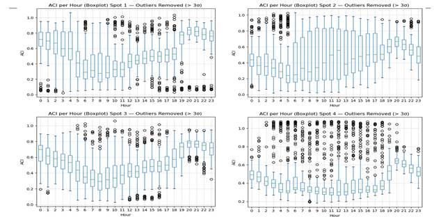
Acoustic indices help quantify different macro characteristics of sites. For example:
- The acoustic complexity index indicates how rapidly sound activity varies over time, and helps contrast dynamic biological activity vs. steady sounds.
- The clustered level of sound quantifies whether the sounds are concentrated in time or spread apart.
- The acoustic diversity index captures how distributed the sounds are across different frequencies.
- The normalized difference soundscape index helps distinguish between natural sounds or human sounds.
- The midfrequency cover similarly helps highlight the degree of activity in the frequency range of insects and birds.
We used data over two weeks to build box-plots of these indices, like the one shown below. Different spots indeed have different profiles.
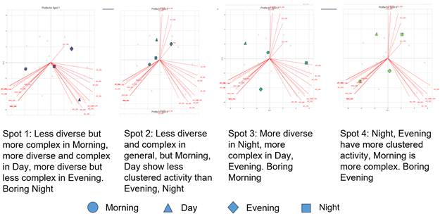
Next, based on these indices, we ran a PCA (Principal Component Analysis) and tried to make sense of it. For each spot, we analyzed it during four periods: morning, day, evening, night.
Access the pipelines
To do such analysis yourself for your sites, please refer to this post on how to set up the CoRE stack ecological monitoring toolkit and the accompanying analysis pipelines.
Github: https://github.com/xHrid/continuous-ecological-monitoring-toolkit
Feedback, issues, ideas, are all welcome. This toolkit will keep evolving, and we’d love to hear how you’re using it in your field projects. Please write to us at contact@core-stack.org
Rajasree Ponnada, Kashvi Khurana, Rachit Aggarwal, Hridayansh Sharma, Aaditeshwar Seth – Indian Institute of Technology Delhi