Next week pest and disease forecasting across Maharashtra
26 Oct 2026
A pest outbreak can damage a crop within a few weeks, and the early signs are easy to miss. Maharashtra already records pest incidence every week through the CROPSAP project, but a report tells you what has already happened. For planning, a farmer also wants to know where a pest is likely to turn up next week.
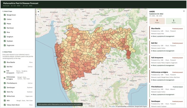
This project builds a forecasting system for exactly that. For ten pests and diseases across eight crops, it shows next week risk on a map of Maharashtra at subdistrict level. A user can click any place to see each pest’s prediction and probability, along with notes on symptoms and management. The dashboard is live at
www.cse.iitd.ernet.in/act4dws5/maharashtra-pest/ and the code is on GitHub.
Figure 1: The dashboard for the week 16 to 23 October 2026, with Aheri subdistrict selected: 9 pests predicted present and 1 absent.
Where the labels come from
We use the weekly pest-report maps of the CROPSAP project, published by ICAR-CRIDA’s Crop Pest DSS. Each map shows one pest in one crop for one week, coloured by severity against the economic threshold level (ETL), with white for no data.
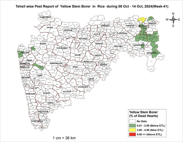
Figure 2: A CROPSAP map for Yellow Stem Borer in rice, week 41 of 2024.
The maps are JPEG images, so we georeferenced one by hand against the Maharashtra boundary and reused its coordinate system, size and extent for all the others. For each of the 359 sub-districts we then took the most common pixel colour inside its polygon. White became class 0 (no pest) and green, yellow and red became class 1 (pest present), so every record is a present or absent label for a crop, pest, year, week and subdistrict.
What the model sees
For each report we take the 90 days of ECMWF ERA5 hourly weather before the report’s end date at that subdistrict. Eight variables are used: dew point, surface pressure, rainfall, soil temperature, solar radiation, and maximum, mean and minimum temperature. Hourly values become daily statistics and then 13 weekly periods, w1 (most recent) to w13 (most distant). That gives 8 × 13 = 104 predictors. Because different pests have different damage period, we test the latest 4, 8 or 13 weeks as separate inputs for each pest.
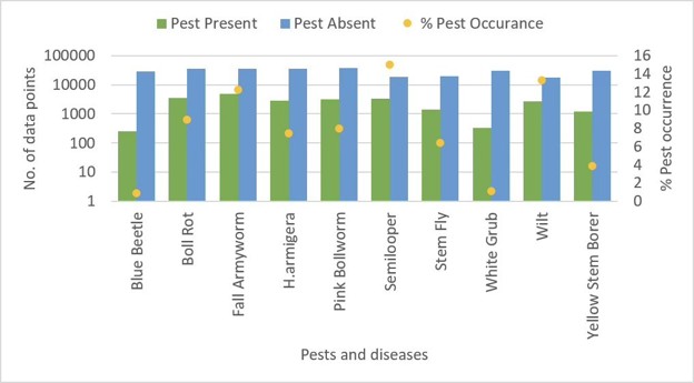
Figure 3: Records with a pest present or absent for each pest (log scale), and the percentage of occurrence.
Pests are rare, so negatives need care
A pest is recorded as present in only 0.8% to 15% of records, about 7.5% overall. A model trained on all of this would learn to say “absent” almost every time.
We handle this in two steps. First, we keep a negative record only where a pest was seen nearby in space, time or crop. We tried three policies: the same subdistrict and week (SYW), the same subdistrict, year and pest (SYP), and the exact subdistrict, week, crop and pest combination (SWCP). Second, we run K-means on the negative records and sample from each cluster in proportion to its size, so the negatives cover many weather conditions rather than a few common ones. Training data is then balanced one to one, while the test data is left naturally unbalanced.
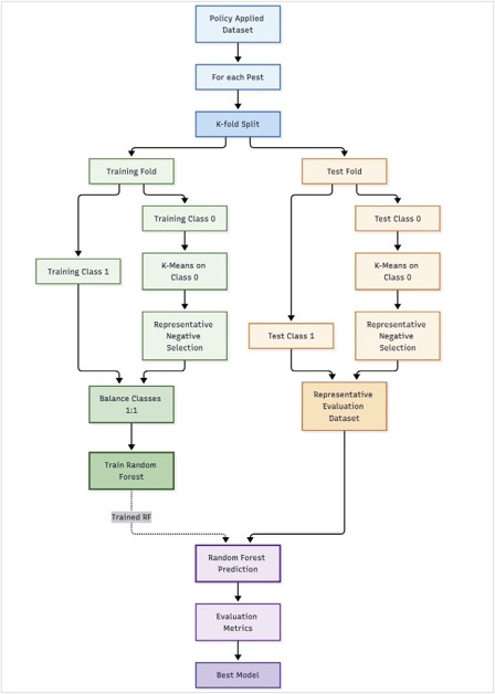
Figure 4: Sampling and model development for each pest.
Models and validation
We train one Random Forest for each of the ten pests, for every combination of three negative sampling policies and three weather windows. That is nine configurations per pest, and for each pest we keep the one with the best mean validation performance. Two validation schemes check how well it generalises:
- Temporal: train on four years and test on the fifth, repeated for each year from 2021 to 2025. This tests an unseen season.
- Spatial: the 359 sub-districts fall into seven normal-rainfall categories, each split into five folds, so every fold spans the same range of rainfall regimes. Training on four folds and testing on the fifth tests unseen but climatically representative sub-districts, which matters for a state-wide system.
Across ten pests, nine configurations, two schemes and five folds, this comes to 900 trained and evaluated experiments. We report accuracy, precision, recall and F1-score.
From model to a daily forecast
The final models are converted into Earth Engine tree representations, one giving the class (0 or 1) and one giving the probability, so they run directly on image pixels inside Google Earth Engine.
Every day at 03:00 IST, an Airflow job starts the forecast run. It builds one continuous daily weather sequence from three sources: ERA5 for history, past ECMWF IFS forecast runs to fill ERA5’s delay of about six days, and the IFS forecast for up to a week ahead. This is converted into the same weekly features used in training, and each pest’s model is applied to every pixel. Results are combined for each sub-district, using the most common class and the mean probability, and published as Earth Engine assets.
The dashboard only reads these published forecasts. This prevents it from triggering expensive forecasting operations.
Using the dashboard
- Open the dashboard in a browser.
- Tick your crops and press Load Forecast Map. Untick any pests you do not want to see.
- Click your place on the map. Zoom with the + and − buttons.
- Read each pest card, which shows its prediction, probability and risk.
- Open “About, symptoms & management” on a card for details.
With one pest selected, red areas show where it is predicted present and green where it is absent. With several, the map combines their predictions, so redder areas have more pests predicted present.
Try it
The dashboard is at www.cse.iitd.ernet.in/act4dws5/maharashtra-pest/ and the code is at github.com/ssjgit08/maharashtraPestDiseaseForecasting.